DDQN/DDDQN example - Cartpole

1. Introduction

본 포스팅에서는 앞선 포스팅에서 다루었던 DDQN과 DDDQN을 Python 기반으로 Cartpole 예제에 적용하여 성능을 분석한다. 전체적인 Cartpole 환경은 DQN 예제 에서 다루었던 환경과 동일하며, DDQN과 DDDQN이 적용됨에 따라 target을 구하는 코드와 학습 모델을 설계하는 코드를 중심으로 다룬다.

2. DDQN

DDQN의 정의에 따라 DQN 예제 포스팅의 DQN Agent 클래스에서 train method를 다음과 같이 변경한다.

class DQNAgent():
    """      
        def __init__():
            ...
    """

    def train(self, batch_size):
        states, actions, rewards, next_states, done_mask = self.memory.sample(batch_size)

        states = torch.FloatTensor(np.array(states))
        actions = torch.tensor(actions).type(torch.int64)
        rewards = torch.FloatTensor(np.array(rewards)).unsqueeze(1)
        next_states = torch.FloatTensor(np.array(next_states))\
        done_mask = torch.FloatTensor(done_mask)

        q_out = self.dqn_net(states.to(device).view(batch_size, -1)) # batch_size by num_actions

        q_a = q_out.gather(dim=1, index=actions.to(device).view(-1, 1)) # batch_size by 1 (q-values for selected actions)

        q_prime_target = self.dqn_target(next_states.to(device).view(batch_size, -1)) # batch_size by num_actions

        # DDQN
        q_prime_net = self.dqn_net(next_states.to(device).view(batch_size, -1)) # main network's q-value (s_prime) 
        a_max_prime = q_prime_net.argmax(1) # main network's greedy action
        max_q_prime = q_prime_target.gather(dim=1, a_max_prime.view(-1, 1)) # target network's q-value applying main network's action

        q_target = rewards.to(device) + self.gamma * max_q_prime_ddqn * (1 - done_mask).to(device).view(-1, 1) # DDQN

        loss = self.criterion(q_a, q_target)

        self.optimizer.zero_grad()
        loss.backward()
        self.optimizer.step()

위의 코드의 line 23~25 까지가 아래 수식과 같은 DDQN에서 Q-value를 구하는 코드이다.

\[Y_{t}^{DDQN} = R_{t+1} + \gamma Q \left( S_{t+1}, \text{arg}\max_{a'} Q ( S_{t+1}, a'| \theta) | \theta^{-} \right)\]

3. Dueling architecture

Dueling architecture를 적용하기 위해, 모델을 정의할 때, value network와 advantage network를 분리해서 설계한다. 기본적인 구성은 DQN 예제 포스팅에서의 DQN Model 과 동일하지만 모델을 정의하는 setup_model() method와 forwad propagation을 위한 forward() method를 dueling architecture에 맞게 수정이 필요하다.

class DQN(nn.Module):
    def __init__(self, num_input_layers, num_output_layers, batch_norm=True):
        super().__init__()

        self.num_input_layers = num_input_layers
        self.num_output_layers = num_output_layers
        self.batch_norm = batch_norm
        self.setup_model()
        self.apply(self._init_weights)
        self._init_final_layer()

    def _init_weights(self, module):
        if isinstance(module, nn.Linear):
            nn.init.kaiming_uniform_(module.weight.data, nonlinearity='relu')
            if module.bias is not None:
                nn.init.constant_(module.bias.data, 0)
        elif isinstance(module, nn.BatchNorm1d):
            nn.init.constant_(module.weight.data, 1)
            nn.init.constant_(module.bias.data, 0)

    def _init_final_layer(self):
        nn.init.xavier_uniform_(self.layer3_val.weight.data)

    def setup_model(self):
        self.layer1 = nn.Sequential(nn.Linear(self.num_input_layers, 32), nn.BatchNorm1d(32), nn.ReLU())
        self.layer2 = nn.Sequential(nn.Linear(32, 64), nn.BatchNorm1d(64), nn.ReLU())
        self.layer3 = nn.Linear(64, self.num_output_layers) # Advantage network
        self.layer3_val = nn.Linear(64, 1) # Value network

    def forward(self, x):
        x = self.layer1(x)
        x = self.layer2(x)

        adv = self.layer3(x)
        val = self.layer3_val(x)
        x = val + adv - adv.mean(1, keepdim=True) # Average aggregation

        return x

    def greedy_action(self, state):
        out = self.forward(state)
        return out.argmax().item()

위의 코드에서 line 27~28이 dueling architecture에서 advantage network와 value network를 정의한 코드이고, value network의 output이 스칼라가 되는 것을 확인한다. 한편 line 34~36은 dueling architecture에서 아래와 수식처럼 average aggregation 을 적용하여 forward propagation을 구현된 내용이다.

\[Q(s, a | \theta, \alpha, \beta) = V(s| \theta, \beta) + \left( A(s, a| \theta, \alpha) - \frac{1}{| \mathcal{A} |} \sum_{a'} A(s, a' | \theta, \alpha) \right)\]

4. 코드 실행 결과

본 포스팅에서 언급한 DDQN과 Dueling architecture와 관련된 코드 이외의 나머지 환경은 모두 DQN 예제에서 다루었던 코드와 동일하다.

4-1. DDQN

DDQN을 적용한 경우, 학습 episode 동안 누적된 보상에 대한 결과를 출력하면 다음과 같다.

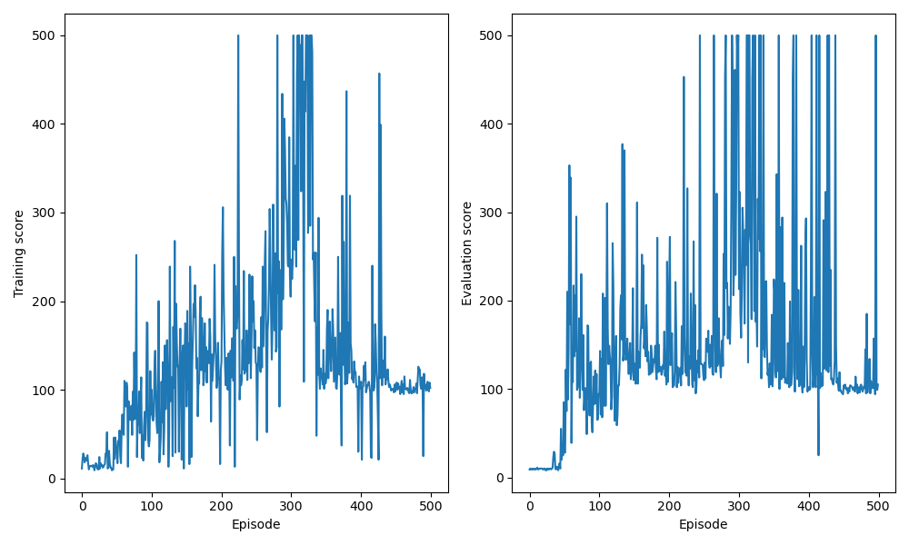Cartpole DDQN results

연산 환경에 따라 출력되는 결과는 상이할 수 있다.

4-2. DDDQN

DDQN에 Dueling architecture를 추가하여 DDDQN을 걱용한 경우, 학습 episode 동안 누적된 보상에 대한 결과를 출력하면 다음과 같다.

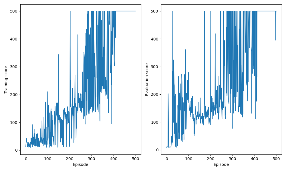Cartpole DDDQN results

연산 환경에 따라 출력되는 결과는 상이할 수 있다.

4-3. 결과 해석

Cartpole과 같이 단순한 환경에서도 target을 구하는 방식의 수정과 학습 모델 구조 개선을 통해, 기본적인 DQN 환경에서의 학습 결과보다 DDQN, DDDQN으로 갈수록 학습 안정성과 성능이 향상되는 것을 확인할 수 있다. 이와 같은 사실을 이용하여 복잡한 환경에서도 DDDQN 적용을 통해 성능 향상을 기대할 수 있다.